


In this post, I’ll talk about an idea called partial measurement from the field of quantum computing. It’s a beautiful idea that you can totally grasp right now, even if you know nothing about quantum computing.
To set the stage, let’s see the basic idea in an everyday world. Suppose that each week, I load up my closet with many shirts of an identical color. I can depend on that. But then I completely forget which color I chose this week. Let’s say that I open the closet, close my eyes, take out one shirt, and close the closet. I open my eyes and look at the shirt: it’s blue. Not only do I know that this shirt is blue, but I also know, for sure and without looking, that all the other shirts in the closet are blue. They must be, because that’s the only possibility consistent with the color I observed.
That’s the basic idea, but it becomes a whole lot more interesting in the quantum world, because quantum measurement is nothing like looking at a shirt. To look at this idea we won’t need any math or any physics. If your imagination is turned on, you have everything you need.
The first part of this post describes what happens when we measure a quantum bit. The second part describes the elegant idea of partial measurement. Throughout, I’ll keep things simple and focused, but I won’t cheat and I won’t tell you anything that’s incorrect. This is the real deal.
Quantum Measurement
Let’s begin with the nature of a single quantum bit (also called a qubit, pronounced Q-bit). Qubits are real things that are used by real quantum computers all the time to do their work, but they’re so small that we can’t see them directly. To figure out how they behave in different situations, we need to put them in those situations and see what happens. That is, we run an experiment that does something to a quantum bit, we see what happens as a result, and that’s how we learn what quantum bits do in different situations.
Over many years and an enormous number of careful experiments, we’ve found that quantum bits don’t work like the stuff we’re used to. Which isn’t all that surprising, since they occupy a realm that is so tiny it feels foreign. Foreign ideas can be unsettling on first contact. For example, to medieval Europeans, elephants were little more than rumors. The notion that some animal could use its nose to pick up things was shocking and weird. But elephants became natural and familiar with time and experience.
So it is with quantum bits. The simplest and most effective way anyone has found to represent them is completely unlike how we think of objects we’re used to, like apples or dogs or mountains. They’re not things in that way, and can feel like the mysterious and perplexing elephants on first exposure.
A key quality of a qubit is revealed by measurement. Let’s look at this idea first in the world we’re used to. Suppose you tell me that you’re holding either a cherry or a blueberry in your closed hand, and you ask me to guess which it is. Before you open your hand, I believe there really is either a cherry or blueberry there. Whatever is in your hand is already one or the other before you show me. Before you open your hand, my inability to say which fruit you’re holding is not due to the fruit being ambiguous in some way. It has a complete, specific identity. The problem is that I’m ignorant of that identity.
A quantum bit is different. Before we observe it, nobody can say what the measurement will reveal. The problem is not like the fruit, where it was our lack of knowledge that held back our prediction. In the quantum case, the object really does not “make up its mind” about what it will be until the moment we make a measurement. Somehow, the thing in your hand is not a fruit yet, but the moment we look at the thing, it becomes a cherry or a blueberry. To see this more clearly, let’s break down quantum measurement.
One thing we’ve learned from a vast number of experiments is that we can only make quantum measurements that have two possible results. You can certainly imagine all kinds of measurements that could return three, four, or any number of values, but for reasons we don’t understand, Nature just doesn’t work that way. When we measure a qubit, we always get back one of two possible outputs, and that’s it. That’s always how it works. So whatever our measurement device is, we can always think of it as a box with two lights on the front. For any measurement, exactly one of the lights turns on.
We can give any names we like to these two possible results: positive and negative, or inside and outside, or yes and no, but most often we name them 0 and 1. So whatever our measurement device is, we can imagine it has two lights on the front labelled 0 and 1. Now we can say that the result of measuring a qubit is just a classical bit (also called a conventional bit) that’s either 0 or 1.
Another way to think of this is to put the burden on the questions we can ask, rather than the possible answers. In that case, we could say that we can only ask questions with two possible results, such as “Is the qubit electrically charged or not?” or “Is it spinning clockwise or counter-clockwise?” We usually abstract away the specifics and say that we can only ask questions that return the answers 0 and 1.
Experiments have shown that if we measure a 0, then further examination always shows that the qubit really is in the state that produces a 0 (we call that state 0). And if we measure a 1, the qubit really is in state 1. That’s reassuring.
But up until the instant of the measurement, the property we’re measuring for this quantum bit is not already in either state 0 or state 1. It’s also not in both states. The whole question of state is actually irrelevant, because the best way anyone has found of representing a property of a qubit before measuring it is that it’s an abstraction: it’s a list of numbers. For this discussion, we can think of this as a list of two small numbers. Everyday, normal numbers that are fractions between 0 and 1. Just how a physical object holds a list of numbers is still a mystery.
These two numbers are the probabilities of our seeing a 0 or 1 on the meter when we make a measurement. To see what that means, I’ll break this up conceptually into 4 steps that happen whenever we make a measurement. I’m listing them here as a sequence, but as far as we know, all of this happens simultaneously and instantly. When we make a measurement:
The universe somehow looks at the property we’re measuring for this quantum bit. Right now all we can say about this property is that it’s a list telling us the probability of ultimately measuring a 0 and the probability of measuring a 1. The qubit is not in either state, and it’s not somehow in “both” states. Asking about its state doesn’t mean anything. A qubit is a thing, like a cherry, but the property we’re testing for is not yet defined. The problem isn’t our ignorance. The state is really undecided, and in its place is a list of probabilities.
Nature picks a final result of either state 0 or state 1 according to the qubit’s probabilities. We fundamentally cannot predict which of the two states Nature will pick. Suppose the probability of measuring a 0 is 0.4, and the probability of measuring a 1 is 0.6. When we measure any single qubit, we get back 0 or 1. If we make a huge number of qubits with these same probabilities, and we measure all of them, we’ll find that roughly 40 percent of them will produce a result of 0, and the remaining 60 percent will produce a 1, but for any specific qubit, we cannot predict if the measurement will be 0 or 1.
Once Nature chooses 0 or 1 for this qubit, the physical object then becomes that state. It is now spinning clockwise or counterclockwise, or it now does or does not have an electrical charge, and so on, for whatever attribute we measured. The qubit switches from representing this property as an abstract list of two probabilities into a specific state, becoming like the things we’re used to. We don’t know how this happens.
Our measurement device sees the property of the quantum bit, which is now definitely in either state 0 or state 1, and presents the corresponding number to us as output.
We say that steps 2 and 3 describe the process of the quantum bit collapsing from its list of probabilities to a single, specific state. Once it’s collapsed and the property takes on a state, it stays there forever, unless we deliberately manipulate it. It doesn’t ever spontaneously go back to being a list, or change its state.
That’s quantum measurement in a nutshell. To recap, a property of a quantum bit starts out as a list of two probabilities, and when we measure it, it unpredictably becomes one or the other based on those probabilities and stays that way. We have no control over this process. The point of quantum computing is to change the lists of probabilities on the quantum bits we’re using so that, when we do ultimately measure a bunch of them, we’re likely to get back a list of 0 and 1 values that are useful.
Now that we know the outlines of measurement, let’s go back to the shirt closet and look at partial measurement.
Partial Measurement
The shirt closet story is more interesting in quantum land because before we open the closet, not only do we not know what color the shirt will be when we look, but the shirt itself doesn’t “know,” either! It only becomes a specific color when we look at it.
Let’s take this into quantum computing, where we usually work with groups of qubits. We’ll see that measuring just one or more of the qubits will cause them to collapse, and the other qubits will necessarily collapse into only those states that are compatible with what we’ve already measured.
Let’s start with an everyday analogy. Suppose I tell you that I have a piece of fruit on my kitchen table. Without more information, that could be almost any kind of fruit imaginable. Then I tell you that it’s round like a ball. Now you know it can only be a fruit that’s compatible with that information: an orange or a grape, for example, but not a banana or a pear. Or I could instead say that it’s red, and now you know it could be an apple or a strawberry, but not a fig or a cantaloupe.
The key thing is that knowing some information about the fruit enabled you to eliminate every fruit that is not compatible with the information I provided. The remaining possible fruits are only those that are compatible with what I’ve told you. That’s the essential idea behind partial measurement.
To expand the idea, let’s switch from guessing fruit to setting up a clothes-washing machine.
Imagine a quantum computer that has 5 qubits. If we measure each of the qubits individually, we can write down all five results one after the other, such as 01001. We can interpret that string of digits any way we like. Often we think of it as a binary number (here it’s the decimal number 17) but it can be lots of other things.
Let’s interpret this string as a sequence of three instructions for how to set up a washing machine in order to do a load of laundry. We tell our quantum computer about the things we want to wash, it runs an algorithm, we measure the qubits, and that bitstring tells us how to set up the water temperature, the load size, and whether or not to enable the slower but more efficient energy-saver mode.
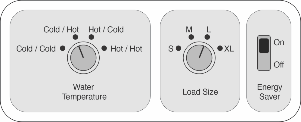
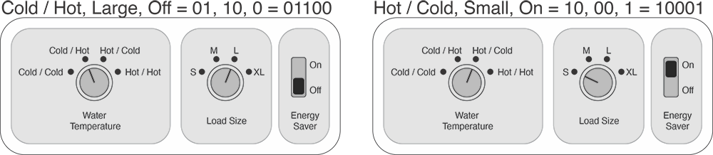
The first two bits can take on any one of the four bitstrings 00, 01, 10, and 11. This means they can tell us which of four choices to make. We might use this to select one of four water combinations in the two phases of wash: 00=cold/cold, 01=cold/hot, 10=hot/cold, and 11=hot/hot. The next two bits tell us the load size: 00=small, 01=medium, 10=large, and 11=extra-large. The final bit is either a 0 or 1, so it can indicate one of two choices: whether the energy-saver mode is 1=on or 0=off. This gives us 32 bitstrings, or 32 possible ways to set up the washing machine. Here are two examples.
Now suppose that our machine is old and breaking down, and some parts have just given up. It cannot switch temperatures between cycles, leaving us with only cold/cold and hot/hot. The motor isn’t strong enough to handle large and extra large if the water is hot. Also, the energy-saver mode is broken. If we tell the quantum computer about these limitations, when we measure an output we should get only one of the six available results: cold/cold with any size load and no energy saver, or hot/hot with small and medium loads and no energy saver.
Here are all six of the states that the quantum computer can produce as an output:
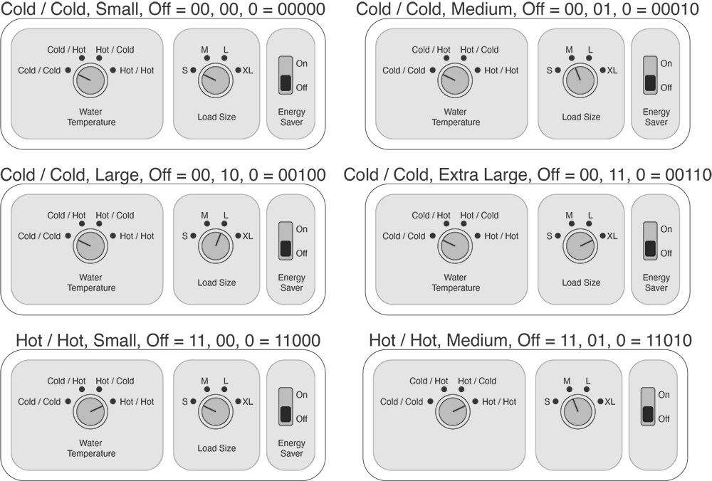
This is a perfect time to use partial measurement! Suppose I measure the first qubit and get a 0 (meaning cold water). Then I immediately know, without measuring anything else, that the second qubit will also give me a 0. It simply can’t be a 1, because the list of six possible states has no entries starting with 01.
One measurement has revealed the state of two qubits!
Suppose that instead my measurement of the first qubit returns a 1. In this case, I’ve learned about two qubits, because when the first bit is 1, the second must also be a 1, and the third bit must be 0. If I make one measurement on the first qubit and get a 1, I know the state of three qubits in total!
On the other hand, If that first bit is a 0, then I don’t learn anything about the third bit, because it can still be either 0 or 1. I need to measure it to find out what it is.
In short, learning about the state of one qubit tells us something about other qubits, because the measurements we make from them ultimately must be part of one of the available states that is compatible with what we’ve already measured.
Learning the states of other qubits in this indirect way is a wonderful tool. For one thing, it means that we can build simpler quantum algorithms, since after the measurement we will have fewer possible states to process.
I gave a hands-on class in quantum teleportation at the SIGGRAPH 2026 computer graphics conference in Los Angeles this July, and afterwards some people in the class asked me about the partial measurement step in the algorithm. I necessarily had to give them brief answers, but I promised to give a fuller answer later, and here it is. For this quick explanation, I’ll assume that you know about the teleportation algorithm, and also the quantum phenomena of superposition and entanglement (if you don’t, you can safely skip the next paragraph).
Just before Alice measures her two qubits, Bob’s qubit is in a superposition of four states, each of which can be written as the tensor product of two states (each either ket 0 or ket 1) and a variation of the state Alice wants to move onto Bob’s qubit. When Alice measures her two qubits (that is, she does a partial measurement of the entire system of 3 entangled qubits), the measurement device returns two classical bits. Because Alice’s qubits have collapsed, Bob’s superposition collapses to the single state that is consistent with Alice’s measurements. Once Alice tells Bob what she measured, Bob knows which variation of Alice’s state he has, and what gates to apply to get back the original state.
Wrapping Up
Partial measurement really means nothing more than “measure some of the qubits.” In some situations, this can reveal information about the other qubits, or eliminate some of their possible states, because ultimately when we measure them we can only get results that are consistent with the first set of measurements. We can exploit this information to make more interesting or more efficient quantum programs.
I told you partial measurement was simple, and now you know why it’s also powerful. Hence, elegant!
If you’d like to get into the details of this idea and other aspects of quantum computing, there are tons of resources available. In particular, I invite you to check out my book “Quantum Computing: From Concepts to Code” from No Starch Press, Amazon, your library, or your favorite bookstore.
Hey you promised me that you’d show me your closet of lovely shirts and then suddenly I’m doing your laundry!? You sly fox you! 😃